Classification of Iris Flower Based on Sepal Length and Petal Length Using Support Vector Machines (SVMs)
The goal was to comprehend the mathematical formulation of Support Vector Machines (SVM) as an optimization problem and acquire practical experience by implementing SVM using pre-built functions from the scikit-learn library. To achieve this objective, a project was undertaken to classify the Iris flower into one of three classes—Iris setosa, Iris versicolor, and Iris virginica—based on the sepal length and petal length of the flower. For this purpose, three SVMs were established, each employing distinct kernels and inequality constraints, effectively addressing the specified task. The design of the SVM and the optimization of the SVM were executed using the SVC function from scikit-learn, a machine learning library, and the results from the three configurations were compared and evaluated for accuracy.
SVM Based Categorization
The idea behind SVM is to find the “best” hyperplane that categorizes the input data containing the labels. To this purpose, we can formulate a convex constrained optimization problem and the solution to this optimization problem gives the hyperplane that can be used to categorize the input data into classes based on the labels.
Given the input data with labels, a regularization parameter C and a kernel, $K: \mathbb{R}^N \times \mathbb{R}^N \rightarrow \mathbb{R}$, the dual soft margin SVM optimization problem is:
\[\begin{align*} & \min \limits_{\alpha \in \mathbb{R}^N} &&\frac{1}{2} \sum_n \sum_m \alpha_n \alpha_m K(x_n,x_m) y_n y_m - \sum_n \alpha_n \\ &\text{subject to} &&0 \leq \alpha_n \leq C \qquad \forall \quad 1 \leq n \leq N \\ & &&\sum_n \alpha_n y_n = 0 \end{align*}\]Upon solving the above optimization problem for the optimal solution $\overline{\alpha} \in \mathbb{R}^N$, we can define a decision function $f:\mathbb{R}^N \rightarrow \mathbb{R}$ such that
\[\begin{align*} f(x) := \sum_n \overline{\alpha}_n y_n K(x_n,x) + b \end{align*}\]Since there are multiples classes in the input data, the SVC function uses “one vs one” approach for classification.
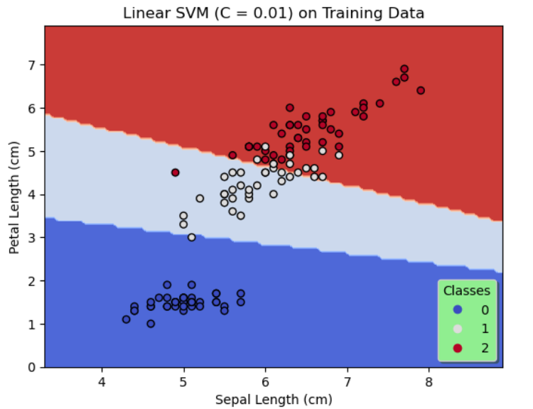
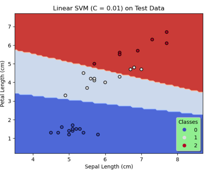
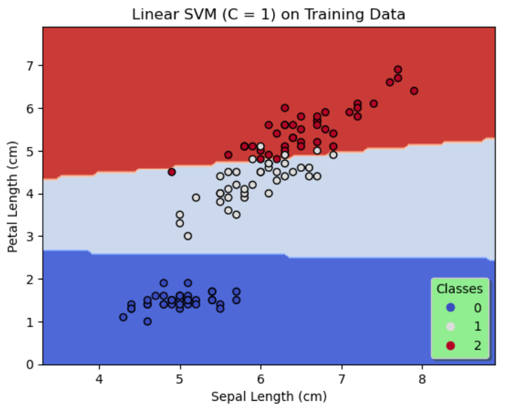
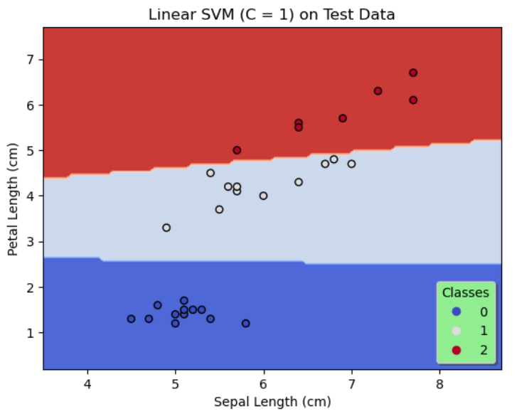
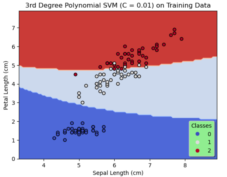
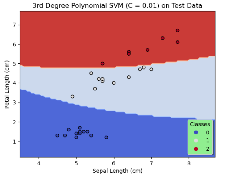
On the whole, SVMs of 3 configurations are designed. The first 2 configurations use a linear kernel with the regularization parameter, C chosen as 0.01 and 1 respectively and the third configuration uses a degree 3 polynomial kernel with $C = 0.01.$
In configuration 1, $K(x,y) = \langle x,y \rangle$.
The configuration 2 is similar to the configuration 1 except that C is set to 1.
In configuration 3, $K(x,y) = (\gamma \langle x,y \rangle + r)^3$ where $\gamma, r$ are set to default values of the arguments of the SVC function.
Results
| Configuration 1 | Configuration 2 | Configuration 3 | |
|---|---|---|---|
| Training Data | 87.5% | 94.2% | 95% |
| Test Data | 90% | 100% | 100% |
Discussion
By comparing the results of the first 2 configurations shown in figures 1 & 2, it is evident by decreasing regularization, that is, by increasing C to 1, the accuracy on the training data and the test data is significantly improved. Likewise, we see a further increase in the accuracy on the training data and a 100% accuracy on the test data as shown in figure 3 when a degree 3 polynomial kernel is used although C = 0.01, that is more regularization is allowed. This seems reasonable since a higher degree polynomial is used as a kernel in configuration 3.
The table above shows the comparison of levels of the final accuracy achieved on the training data and the test data for the 3 configurations.
In all three configurations, by observing the figures 1, 2 & 3 there is no evidence of overfitting.