Dense Neural Network Based Categorization of Iris Data
The primary goal of this project was to thoroughly understand the core principles of neural networks, involving the implementation of four fundamental steps: initialization of the weights and biases, feedforward and backpropagation algorithms, and optimization using stochastic gradient descent. A small-scale project to classify Iris flowers into three classes based on specific characteristics was undertaken. A dense neural network for this task was developed and implemented in Python, utilizing a dataset from https://archive.ics.uci.edu/ml/datasets/Iris. The secondary objective was to gain hands-on experience with neural network design and optimization using the Keras library. Stochastic gradient descent (SGD) algorithm with a default learning rate of 0.01 was employed for optimizing the weights and biases.
Dense Neural Network Based Categorization
On the whole, 3 dense neural networks of different configurations are designed. Every configuration has an input layer has 4 neurons since there are 4 characteristics associated with each observation. Likewise, the output layer has 3 neurons since there are 3 classes of the Iris flower. Also, the activation function of the neurons in every configuration is a Sigmoid, that is, $\displaystyle \sigma(z) = \frac{1}{1+e^{-z}}$.
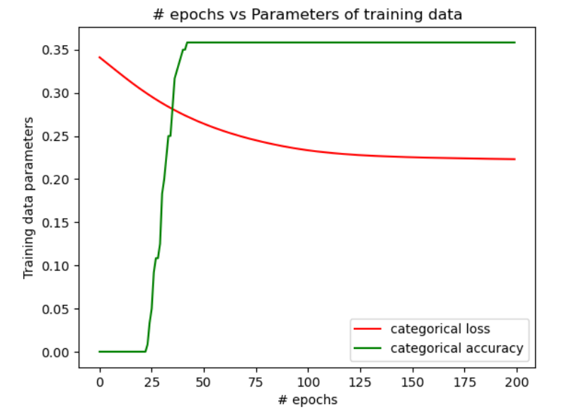
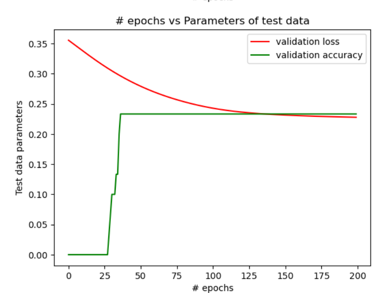
In configuration 1, there is 1 hidden layer consisting of 4 neurons. Hence, there are 35 parameters that could be optimized. The cost function is defined to be the mean-squared error, that is,
\(\displaystyle C =\frac{1}{2n}\sum_x ||y(x) - a^L(x)||^2\).
The algorithm chosen to find the optimal weights and biases is the Stochastic Gradient Descent (SGD) with a default learning rate of 0.01. The training inputs and training targets are split into a batch size of 10 and the stopping criteria for convergence is set to 200 epochs.
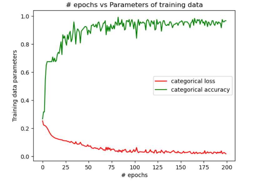
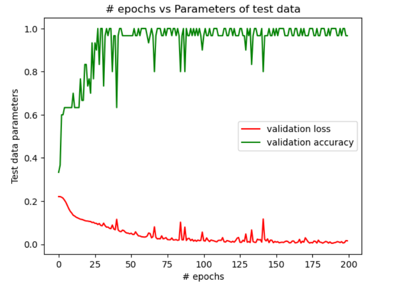
The configuration 2 is similar to configuration 1 except that the learning rate for the SGD is set to 1.
In configuration 3, the cost function is defined as the cross entropy, that is, $\displaystyle C =-\frac{1}{n}\sum_x \big[ y\ln{a} + (1-y) \ln{(1-a)} \big]$ and there are 10 neurons in the hidden layer. So, there are 83 parameters that could be optimized. The learning rate for the SGD is set to the default which is 0.01.
NOTE: Given any neuron in the layer l, if it is connected to every neuron in the layer l+1 then such a neural network is called as a dense neural network.
Results
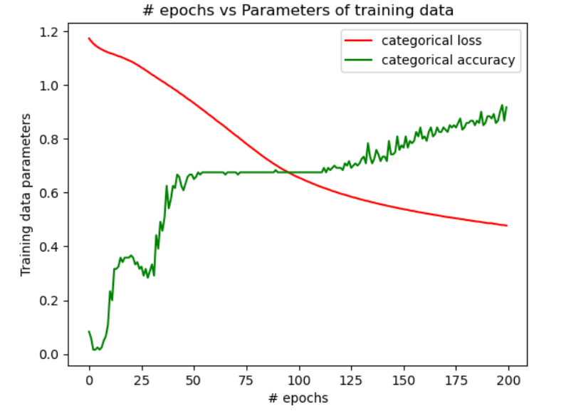
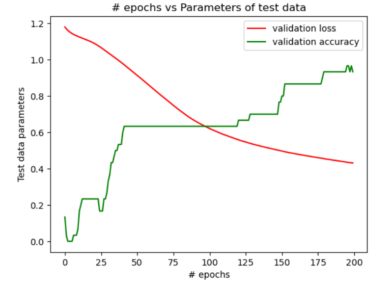
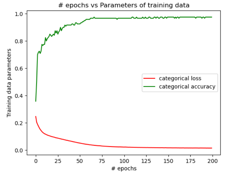
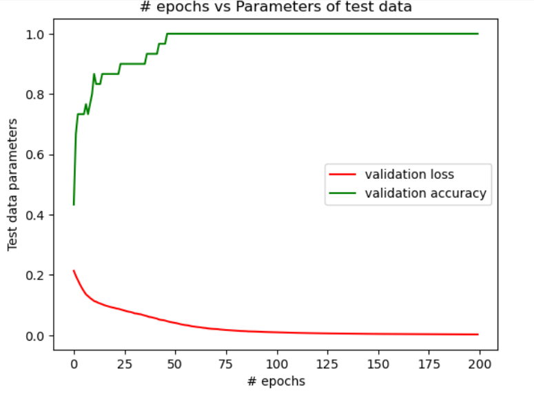
| Configuration 1 | Configuration 2 | Configuration 3 | |
|---|---|---|---|
| Training Data | 35.8% | 97.5% | 85.8% |
| Test Data | 23.3% | 96.6% | 90% |
Discussion
In figure 1, we see that when the NN is designed as per the configuration 1, the accuracy is a constant beyond 50 epochs and doesn’t change with epochs. Also, the accuracy is poor. However, when the NN is designed as per the configurations 2 & 3, there is a major improvement in the accuracy of the training data and the test data as seen in figures 2 & 3. But, by comparing the change in the accuracy with the number of epochs, it is evident from figures 2 & 3 that a higher accuracy is achieved with the least epochs in the configuration 2 when compared with the configuration 3. The table above shows the comparison of levels of the final accuracy achieved on the training data and the test data for the 3 configurations.