Elliptic optimal control problem with control constraints

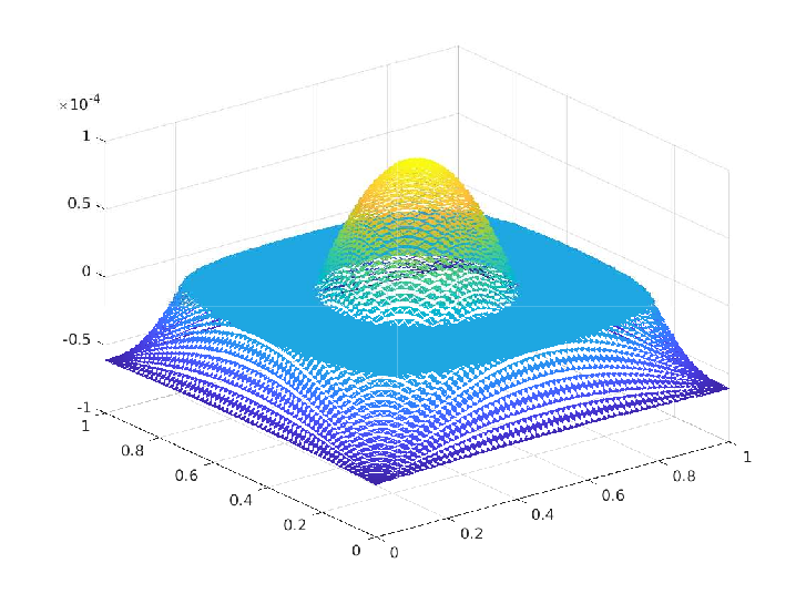
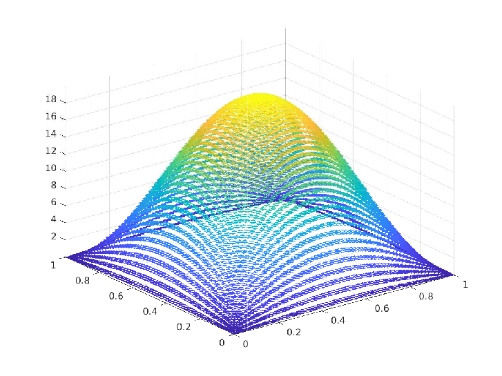
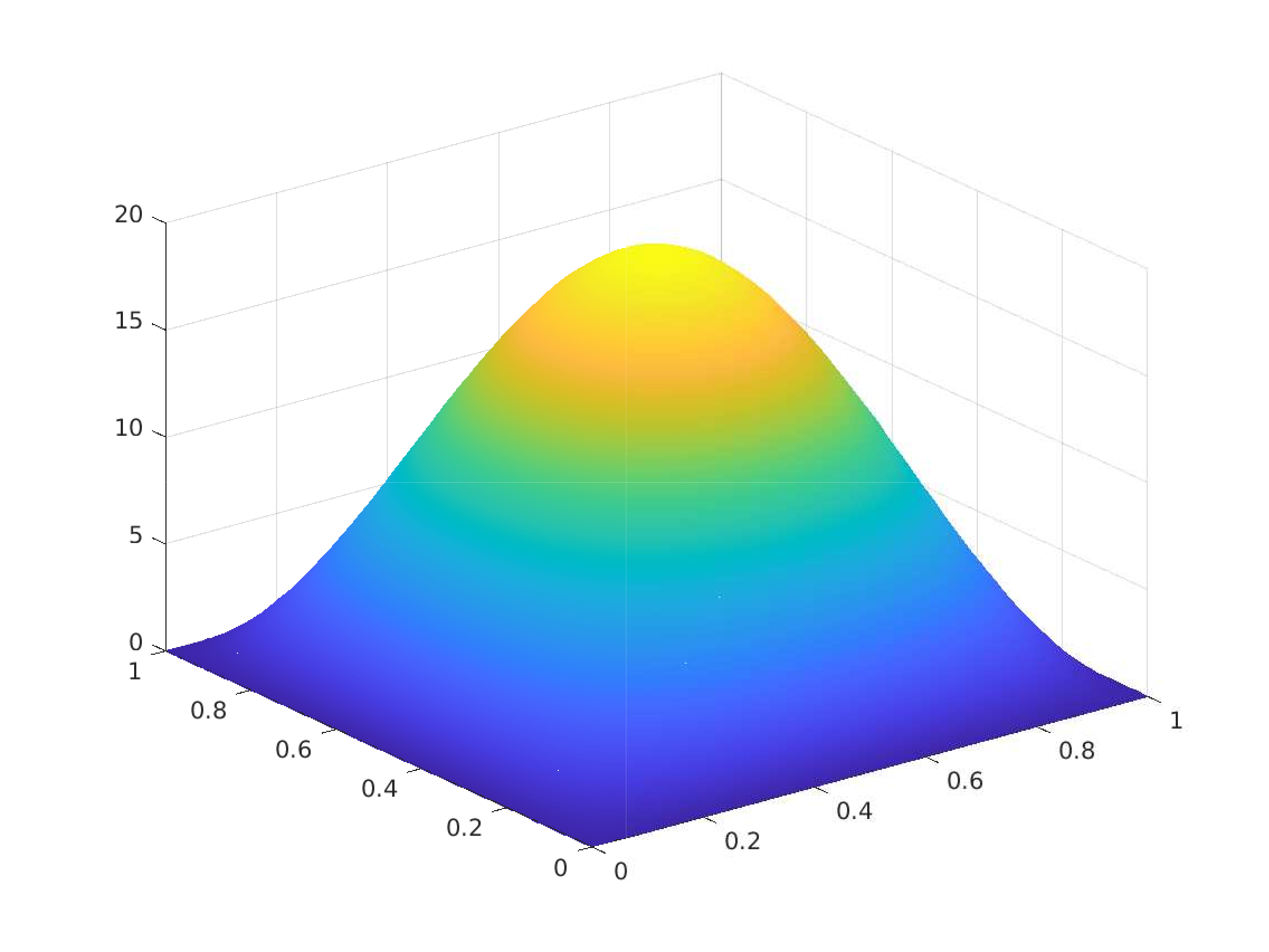
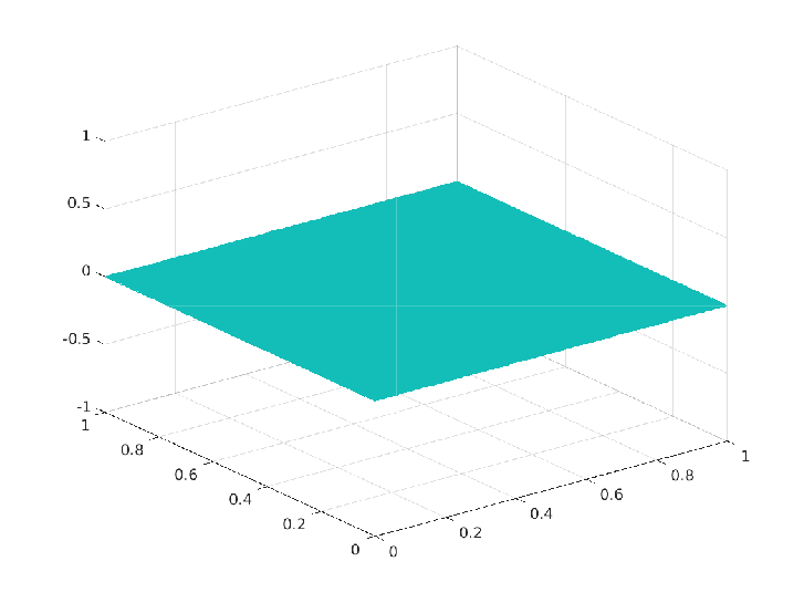
We proposed a numerical scheme to reduce an elliptic optimal control problem with control constraints to a finite-dimensional optimization problem with equality and inequality-type constraints and established the order of convergence of the error as we refine the triangulation of the polygonal domain $\Omega \subset \mathbb{R}^2$.

Let $\Omega$ contained in $\mathbb{R}^2$ be a bounded convex polygonal domain with Lipschitz boundary $\partial \Omega$.

Let $y_d \in L^2(\Omega)$ be the desired state, $u_a, u_b \in \mathbb{R} \cup$ {$\pm \infty$} such that $u_a < u_b$ be given and $\beta > 0$ be a regularization parameter. The elliptic optimal control problem (EOCP) with control constraints in given by

where $U_{ad}$ := {$v \in L^2(\Omega): u_a \leq v \leq u_b$} is a closed convex set, $y$ is the “state” variable, and $u$ is the “control” variable. The constraints on the control variable $u$ are called box constraints. When $u_a = -\infty$ and $u_b = \infty$, observe that $U_{ad} = L^2(\Omega)$. Then, we have an optimization problem with no inequality constraints, which is a special case of the optimization problem under consideration.

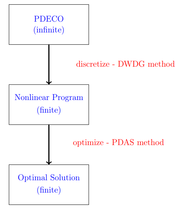
In this project, we aim to obtain an optimization problem with equality and inequality-type constraints in finite dimensions and solve it for the numerical optimal solution. To do so, we replace the infinite-dimensional admissible set, the infinite-dimensional functional, and the infinite-dimensional Laplacian operator with a finite-dimensional admissible set, a finite-dimensional functional, and a discrete Laplacian operator, respectively. Note that the finite-dimensional admissible set is spanned by the discontinuous piecewise polynomials with respect to the underlying triangulation of the polygonal domain $\Omega \subset \mathbb{R}^2$ and the discrete Laplacian operator is constructed using the dual-wind DG (DWDG) method. The discrete KKT system is derived using this finite-dimensional optimization problem, and the PDAS algorithm is then utilized to find the numerical optimal solution in finite dimensions that satisfies the discrete KKT system. Later, we show that this finite-dimensional optimal solution eventually converges to an infinite-dimensional optimal solution as we refine the triangulation of the polygonal domain $\Omega$. Additionally, we establish the orders of convergence in $L^2$ and energy norms.

Here is a lecture on brief introduction to PDE constrained optimization by Dr. Stegan Volkwein

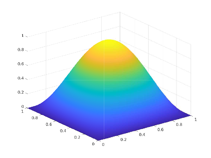
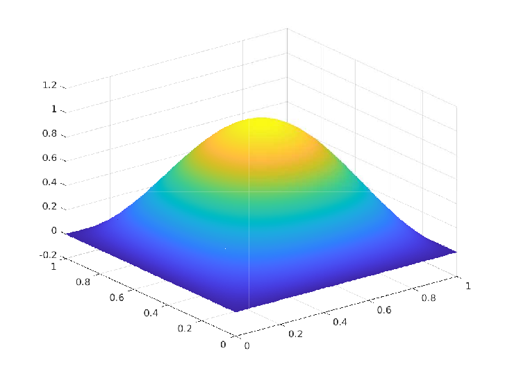
Numerical Experiment - 1: Trivial box constraints on the control

\(\Omega = [0,1]^2, \, u_a = -\infty, \, u_b = \infty, \, y_d = (1+4\pi^4) \sin(\pi x_1) \sin(\pi x_2)\)

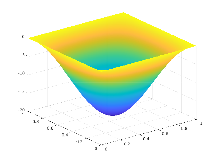
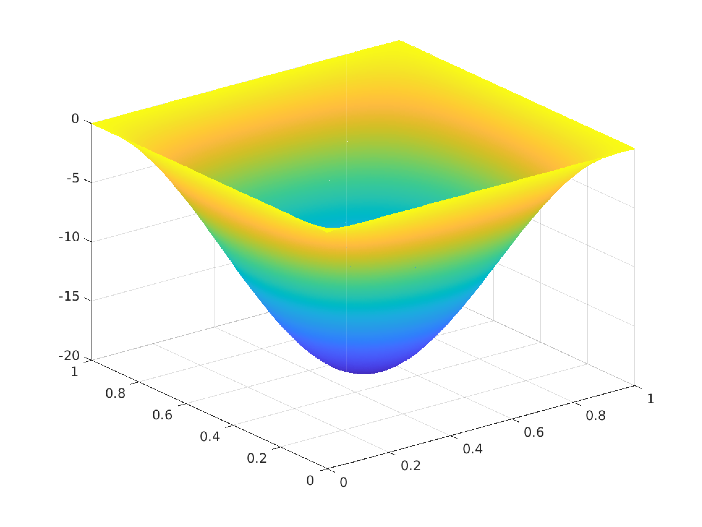
Exact solution $(\overline{y},\overline{p},\overline{u}) \in H^1(\Omega) \times U_{ad} \times H^1(\Omega)$:
\(\begin{array}{rrlrrlrrl} & \overline{y}(x_1,x_2) & = & \sin(\pi x_1) \sin(\pi x_2) \\ & \overline{p}(x_1,x_2) & = & -2 \pi^2 \sin(\pi x_1) \sin(\pi x_2) \\ & \overline{u}(x_1,x_2) & = & 2 \pi^2 \sin(\pi x_1) \sin(\pi x_2) \end{array}\)

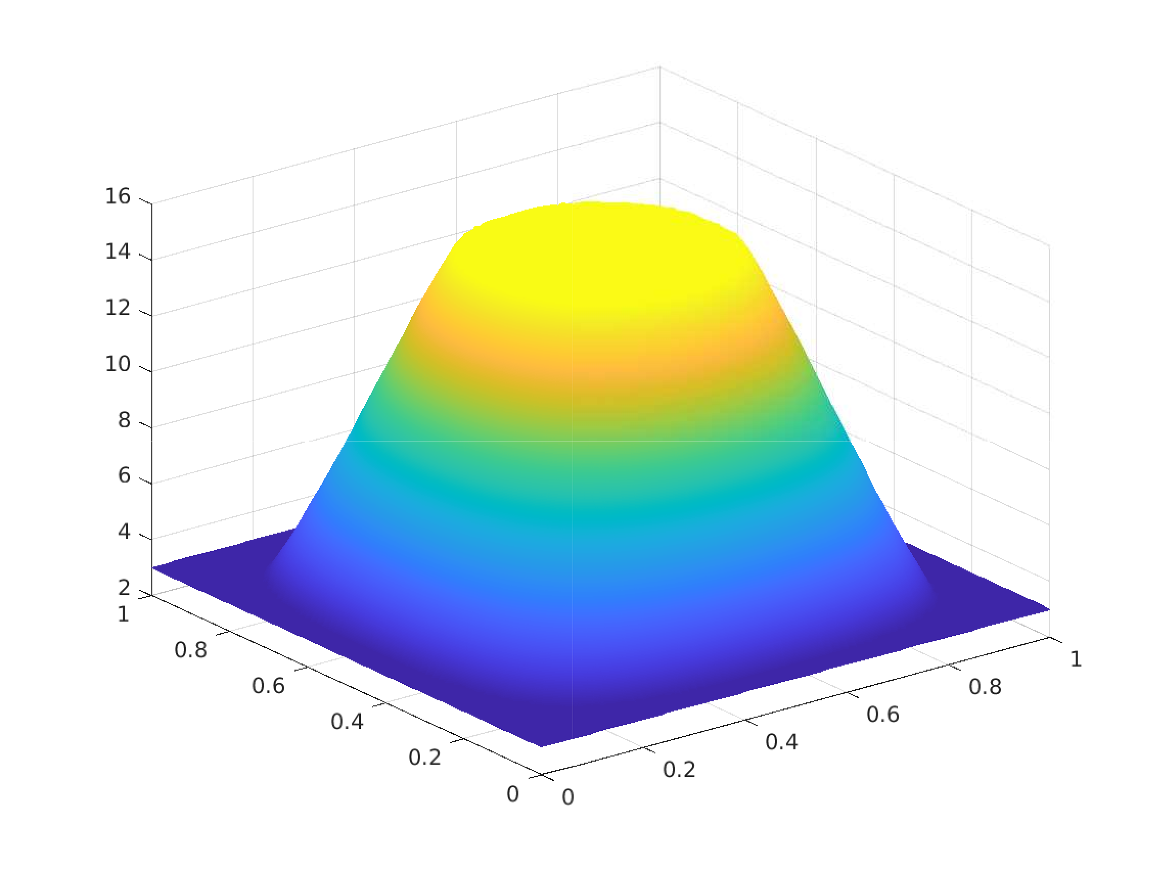
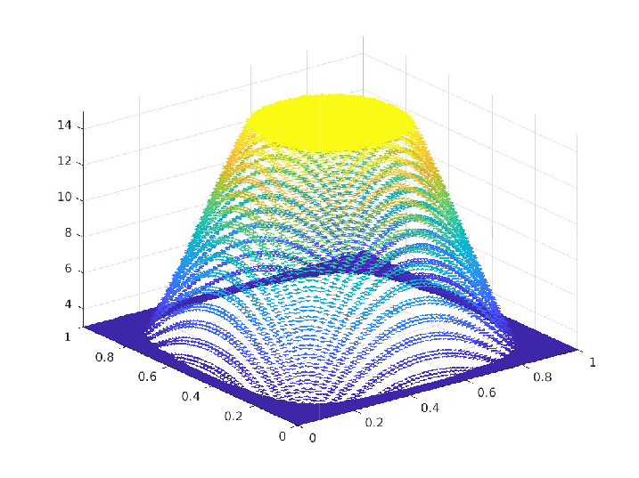
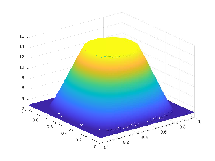
Numerical Experiment - 2: Non- trivial Box constraints on the control

[A Rösch, R Simon (2005)]

\(\Omega = [0,1]^2, \, u_a = 3, \, u_b = 15, \, y_d = (1+4\pi^4) \sin(\pi x_1) \sin(\pi x_2)\)

Exact solution $(\overline{y},\overline{p},\overline{u}) \in H^1(\Omega) \times U_{ad} \times H^1(\Omega)$:
\(\begin{array}{rrlrrl} & \overline{y}(x_1,x_2) & = & \sin(\pi x_1) \sin(\pi x_2) \\ & \overline{p}(x_1,x_2) & = & -2 \pi^2 \sin(\pi x_1) \sin(\pi x_2) \end{array} \\ \begin{array}{rrl} & \overline{u}(x_1,x_2) & = & \begin{cases} u_a, \quad \text{if } 2 \pi^2 \sin(\pi x_1) \sin(\pi x_2) < u_a, \\ 2 \pi^2 \sin(\pi x_1) \sin(\pi x_2), \quad \text{if } 2 \pi^2 \sin(\pi x_1) \sin(\pi x_2) \in [u_a, u_b], \\ u_b, \quad \text{if } 2 \pi^2 \sin(\pi x_1) \sin(\pi x_2) > u_b \end{cases} \end{array}\)