Gaussian Mixture Models (GMMs) Based Density Estimation of US Cities Preferring One Size of Avocados
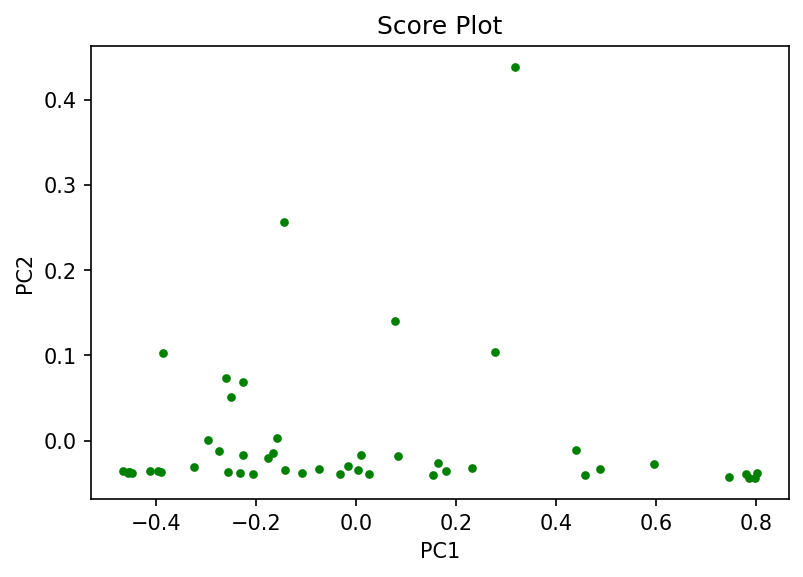
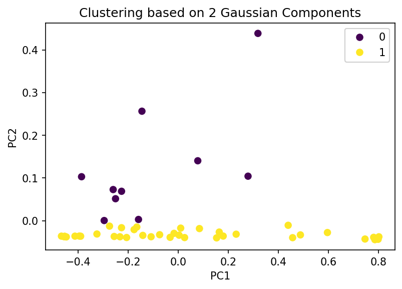
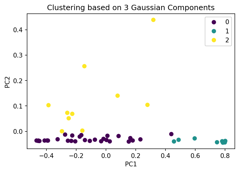
After reducing the dimensionality of the data through PCA, the density distribution of the cities preferring small, medium, or all sizes of avocados, as represented by the score plot, was estimated using GMMs. The expectation maximization (EM) algorithm, an iterative scheme, was used to determine the model parameters. Consequently, the data depicted in the score plot was effectively clustered into three distinct clusters. These clusters represent cities with high sales of small-sized avocados, cities with high-medium sized avocado sales, and cities with outlier sales in large-sized avocados. The project was coded in Python.
GMMs $\&$ EM algorithm
[Deisenroth et al. (2020)]
GMMs
Given a dataset \(\mathcal{X} =\{\boldsymbol{x}_1,\boldsymbol{x}_2,\cdots,\boldsymbol{x}_N\}\) where \(\boldsymbol{x}_n\) are i.i.d for $1 \leq n \leq N$, the goal is to approximate $p(\boldsymbol{x})$ by a convex combination of $K$ Gaussian distributions where $K$ is fixed as an apriori. That is, for a fixed $K$, we want to have $p(\boldsymbol{x}) = \sum_{k = 1}^K{\pi_k \mathcal{N}(\boldsymbol{x}|\boldsymbol{\mu_k},\boldsymbol{\Sigma_k})}$ such that $0 \leq \pi_k \leq 1$ and $\sum_{k=1}^K \pi_k = 1$. Subsequently, we want to determine the parameters, \(\boldsymbol{\theta}:= \{\pi_k,\boldsymbol{\mu_k},\boldsymbol{\Sigma_k}: k = 1,2,\cdots,K \}\) such that $p(\mathcal{X}|\boldsymbol{\theta})$, the likelihood is maximized where
\(p(\mathcal{X}|\boldsymbol{\theta}) = p(\boldsymbol{x_1}|\boldsymbol{\theta}) \times p(\boldsymbol{x_2}|\boldsymbol{\theta}) \times \cdots \times p(\boldsymbol{x_N}|\boldsymbol{\theta}) = \prod_{n = 1}^N p(\boldsymbol{x_n}|\boldsymbol{\theta})\) and $p(\boldsymbol{x_n}|\boldsymbol{\theta}) = \sum_{k = 1}^K{\pi_k \mathcal{N}(\boldsymbol{x_n}|\boldsymbol{\mu_k},\boldsymbol{\Sigma_k})}$.
To simplify, we define $ \mathcal{L} := \log p(\mathcal{X}|\boldsymbol{\theta}) = \sum_{n = 1}^N \log p({x_n}|\boldsymbol{\theta}) = \sum_{n = 1}^N \log \left(\sum_{k = 1}^K \pi_k \mathcal{N}(\boldsymbol{x}_n|\boldsymbol{\mu_k},{\Sigma_k})\right) $ called the log-likelihood. Now, our objective is to maximize $\mathcal{L}$.
EM algorithm
To this end, we use the EM algorithm which is an iterative scheme. By employing EM algorithm, we update one model parameter at a time while keeping the other parameters fixed. So, we define
\(\displaystyle r_{nk}:= \frac{\pi_k \mathcal{N}(\boldsymbol{x}_n|\boldsymbol{\mu}_k,\boldsymbol{\Sigma}_k)}{\sum_{j=1}^K\pi_j \mathcal{N}(\boldsymbol{x}_n|\boldsymbol{\mu}_j,\boldsymbol{\Sigma}_j)}\) called as the responsibility of the $k^{\text{th}}$ Gaussian mixture component for the data point $\boldsymbol{x}_n.$
First, we initialize $\boldsymbol{\mu}_k, \boldsymbol{\Sigma}_k, \pi_k$.
Next, we compute the responsibilities $r_{nk}$ which is called the E-step.
Later, we use the computed responsibilities to re-estimate the parameters $\boldsymbol{\mu}_k, \boldsymbol{\Sigma}_k, \pi_k$. This step is called the M-step.
The E-step and the M-step are run alternately until a convergence criterion is met.
Results
Discussion
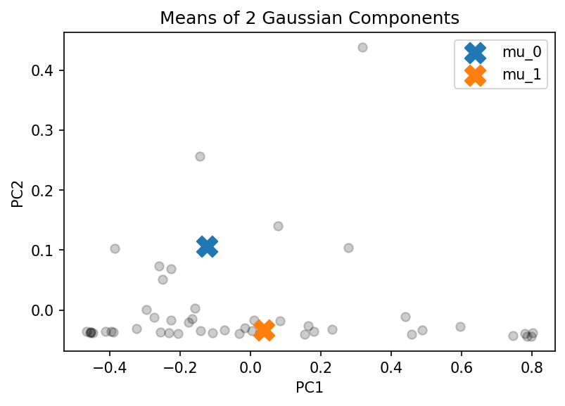
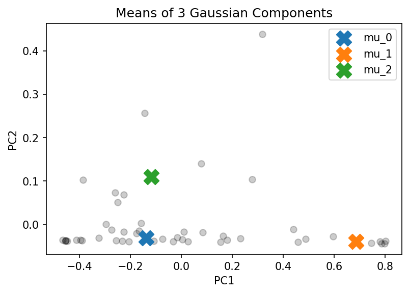
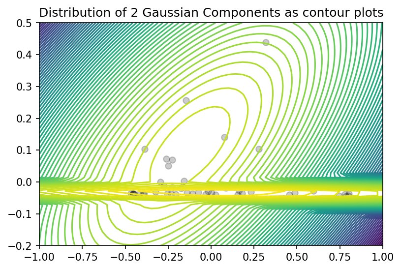
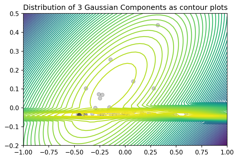
Visually, we can see from the score plot that there are 3 clusters - one at the bottom left, one at the bottom right, and one at the top center. Hence I think choosing to estimate the density with 3 Gaussian components is better in comparison with the density estimation by 2 Gaussian components. When K = 3, the means are at the centers of the 3 clusters we can visually detect where as when K = 2, the data points belonging to the cluster at the bottom has more “concentration” on the left hence $\mu_1$ is not at the center but it is slightly at the bottom left.
In both cases, when K = 2 and K = 3, the clustering at the bottom shows variance of the data along the PC1 direction which is evident by the contour plots of the distributions of GMMs of 2 and 3 components. We can make a similar comment about the clustering at top center.
Evaluation
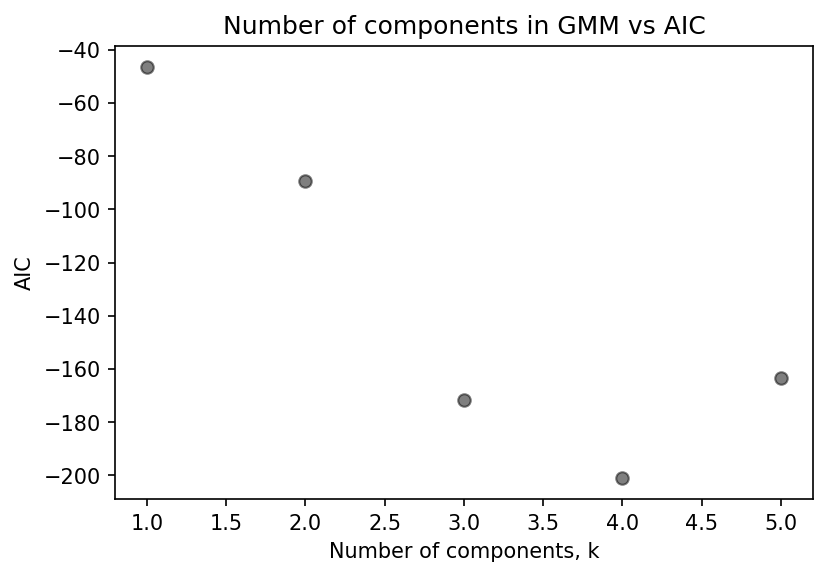
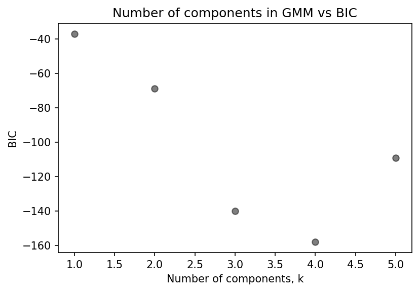
From the plots that show AIC and BIC, we can clearly see the GMM with 4 components has the lowest score. However, the decrease in the score when using 3 components and 4 components is not on par with the reduction in score when using 2 components and 3 components. Hence, we can conclude that using three-component GMM is optimal.
The insights by GMM on this data clearly concur with the insights that we get by visually inspecting the score plot.